Correcting Differential Item Functioning (DIF) Within Multi-Item Scales Using R

Applying a sequential Rasch framework to the Authoritarianism scale from the American National Election Study

Differential item functioning (DIF) is a hidden characteristic often found in the data used to construct multi-item scales. This document provides a tutorial for using R to identify and correct DIF in survey data using the sequential Rasch framework we describe in this article.

For more details, see our paper: Pietryka, Matthew T., and Randall C. MacIntosh. 2022. “ANES Scales Often do not Measure What You Think They Measure.” The Journal of Politics. doi.org/10.1086/715251.

0. Set up

The code in this tutorial requires the following packages and functions:

Show code

# these packages are necessary  
library(dplyr)
library(tidyr)
library(tibble)
library(purrr)
library(readr)
library(TAM)
library(ggplot2)
library(broom)

# these packages are not necessary
# (they are only used to display tables in this tutorial)
library(kableExtra)
library(texreg)

# function to display a data frame as markdown table
display_tab <- function(df){
  df  %>% 
    kbl(digits = 2) %>%
    kable_material(
      c("striped", "hover", "condensed"), 
      full_width = FALSE
      ) 
}

1. Clean the data

The first step is to obtain appropriate data and prepare it for analysis. In this tutorial, we will use the 2016 American National Election Study (ANES), which can be downloaded from www.electionstudies.org.

Data Citation: American National Election Studies, University of Michigan, and Stanford University. ANES 2016 Time Series Study. Ann Arbor, MI: Inter-university Consortium for Political and Social Research [distributor], version 5/2/2017. https://doi.org/10.3886/ICPSR36824.

1.1. Load the data

The data come in Stata format (.dta extension), which we can load in R with the haven::read_dta() function.

Show code

anes <- haven::read_dta("anes_timeseries_2016_Stata12.dta")

1.2. Prepare the variables for analysis

We will examine whether the Authoritarianism scale provides measurement equivalence for comparisons by age. To do so, we use the code below to:

1. construct four dichotomous Authoritarianism items (auth_respect, auth_manners, auth_obed, auth_behave). For each item, respondents choosing the authoritarian response are coded as ones and those choosing the non-authoritarian response are coded as zeros.
2. construct a variable called age measuring each respondent’s age in years.
   
3. construct a three-point grouping variable called age3, which assigns each respondent into one of three age groups of roughly equal size.

This example uses age cutpoints to obtain similarly sized groups but the procedure does not require a specific number of groups, nor must they be similar in size.

Show code

anes_sub <- anes  %>% 
  haven::zap_labels()  %>% 
  # rename variables
  rename(
    case_id = V160001,
    weight  = V160102
  )  %>% 
  # clean the Authoritarianism items (1 = Authoritarian response)
  mutate(
    auth_respect = recode(V162239, `1` = 0L, `2` = 1L, .default = NA_integer_),
    auth_manners = recode(V162240, `1` = 0L, `2` = 1L, .default = NA_integer_),
    auth_obed    = recode(V162241, `1` = 1L, `2` = 0L, .default = NA_integer_),
    auth_behave  = recode(V162242, `1` = 0L, `2` = 1L, .default = NA_integer_)
    )  %>% 
  # create `age3` grouping variable 
  mutate(
    age  = ifelse(V161267c > 0, 2016 - V161267c, NA_integer_),
    age3 = ntile(age, 3)
  )  %>% 
  # extract relevant variables 
  select(
    case_id,
    weight,
    age,
    age3,
    auth_respect,
    auth_manners,
    auth_obed,
    auth_behave
    )  %>% 
  # subset to non-missing on age
  drop_na(age3)
         


# save subsetted data as .rds file
write_rds(anes_sub, "anes_sub.rds")

To follow along with this tutorial, you can download the cleaned data (the anes_sub object, constructed above) here:

Download anes_sub.rds

You can load these data with the readr::read_rds() function:

Show code

# this code assumes you saved `anes_sub.rds` in your current working directory
anes_sub <- read_rds("anes_sub.rds")

2. Estimate the Rasch model

With the data prepared, we fit the initial Rasch model. To do so, we must first extract the scale items.

Show code

item_data_1 <-  anes_sub  %>% select(starts_with("auth_"))
head(item_data_1)

# A tibble: 6 × 4
  auth_respect auth_manners auth_obed auth_behave
         <int>        <int>     <int>       <int>
1            1            1         1           0
2            0            1         0           0
3            0            1         0           1
4            1            0         0           0
5            1            1         1           1
6           NA           NA        NA          NA

We can then estimate the Rasch model with the TAM::tam.mml() function. We specify the following arguments in the functions:

1. the resp argument specifies the scale items for analysis.
2. The irtmodel argument chooses the appropriate model. The TAM::tam.mml() function can fit many types of models other than the Rasch, so we must specify irtmodel = "1PL" to fit the binary Rasch model. The Rasch model is sometimes called a ‘1PL’ or ‘One Parameter Logistic’ model because it has only one parameter per item. The single parameter represents the item’s location on the latent trait.
3. We add sample weights with the pweights argument.
4. We use control = list(progress = FALSE) to reduce the amount of output in the R console.

This tutorial focuses on a scale with dichotomous items, but in the paper we also discuss methods for polytomous items. The TAM::tam.mml() function can fit these models by changing the irtmodel argument to irtmodel = "RSM" for the Rating Scale Model or irtmodel = "PCM" for the Partial Credit Model.

Show code

# set the seed
set.seed(2192343)

# fit the model
rasch_1 <- tam.mml(
  resp = item_data_1,
  irtmodel = "1PL",
  pweights = anes_sub$weight,
  control = list(progress = FALSE)
  )

After fitting the model, one can view the item locations by examining the xsi.item parameter from the model object. Greater values indicate more difficult items.

Show code

rasch_1$item  %>% select(item, xsi.item)  %>% display_tab()

	item	xsi.item
auth_respect	auth_respect	-1.62
auth_manners	auth_manners	-0.99
auth_obed	auth_obed	0.05
auth_behave	auth_behave	0.93

In this case, auth_behave appears to be the most “difficult” item requiring the highest level of Authoritarianism. This difficulty indicates that, on average, a respondent who chooses the authoritarian response on this item has the greatest value of the latent trait compared to those who do not endorse it.

3. Estimate ANOVAs to evaluate differential item functioning (DIF)

Before comparing the age groups on the latent trait, we must examine whether any item exhibits DIF by age. To do so, we fit a one-way ANOVA of each item’s misfit to the model (as residuals from the expected value) on group membership (the age terciles).

3.1 Extract each item’s residuals from the Rasch model

We extract the residuals and merge them with the cleaned survey data, producing a new data frame called anes_resids.

Show code

# extract item residuals
resids_1 <- IRT.residuals(rasch_1)$stand_residuals  %>% 
  as_tibble()   %>% 
  set_names(paste0("resid_", names(.)))
  
# merge with grouping variable, case ID, and survey weights
anes_resids <- anes_sub  %>% 
  select(case_id, weight,age3)  %>%
  bind_cols(resids_1) 

We then tidy the data to make it easier to fit an ANOVA for each item. To do so, we “pivot” the four columns into one “longer” data.frame.

Show code

# tidy the residual data (wide to longer) 
anes_long <- anes_resids  %>%
  pivot_longer(
    c(
      resid_auth_respect, 
      resid_auth_manners, 
      resid_auth_obed, 
      resid_auth_behave
      ),
    names_to = "item", 
    values_to = "residual", 
    )

3.2 For each item, estimate an ANOVA of the Rasch standardized residuals on group membership

One can estimate a single ANOVA as follows:

Show code

# fit a single ANOVA 
anova_1 <- aov(
  resid_auth_respect ~ factor(age3),
  data = anes_resids,
  weights = weight
  )
summary(anova_1)

               Df Sum Sq Mean Sq F value Pr(>F)    
factor(age3)    2   45.4  22.686   38.22 <2e-16 ***
Residuals    3470 2059.4   0.593                   
---
Signif. codes:  0 '***' 0.001 '**' 0.01 '*' 0.05 '.' 0.1 ' ' 1
677 observations deleted due to missingness

We can see that the standardized residuals vary significantly across the groups. If your grouping variable has more than two values, however, you will want to know which groups differ. To answer this question, you can estimate a post-hoc test:

Show code

posthoc <- TukeyHSD(anova_1)
posthoc

  Tukey multiple comparisons of means
    95% family-wise confidence level

Fit: aov(formula = resid_auth_respect ~ factor(age3), data = anes_resids, weights = weight)

$`factor(age3)`
          diff         lwr       upr     p adj
2-1 0.21406746  0.14219142 0.2859435 0.0000000
3-1 0.25770657  0.18568638 0.3297268 0.0000000
3-2 0.04363911 -0.02896268 0.1162409 0.3361306

The post-hoc test indicates that age group 1 differs significantly from age groups 2 and 3, but groups 2 and 3 do not differ significantly from one another.

Before we conclude that this item shows DIF, however, we must first evaluate whether the other items show DIF as well. Any single item showing DIF can create “artificial” DIF in the remaining items.¹ Therefore, the apparent DIF shown above may not be real DIF that needs correcting. We can only tell by examining the DIF for all the items. We do so by first creating a function to fit the ANOVA:

Show code

fit_anova <- function(df){
  aov(
    residual ~ factor(age3),
    data = df,
    weights = weight
  )
}

We can then create a “nested” data frame that we will use to apply the function to each item in the scale. The nested data frame is a data frame that holds other data frames inside. In this case, each row of the data column contains a data frame that includes only the residuals for a single item (along with the grouping variable, case IDs, and weights):

Show code

anes_nested_1 <- anes_long  %>% 
  group_by(item)  %>% 
  nest()

anes_nested_1

# A tibble: 4 × 2
# Groups:   item [4]
  item               data                
  <chr>              <list>              
1 resid_auth_respect <tibble [4,150 × 4]>
2 resid_auth_manners <tibble [4,150 × 4]>
3 resid_auth_obed    <tibble [4,150 × 4]>
4 resid_auth_behave  <tibble [4,150 × 4]>

We can then apply the ANOVA function we created to each of the rows in our nested data frame. To do so, we use the purrr::map() function. We can then use the broom::tidy() function to format the ANOVA results, making them easier to read. Finally, we must recognize that we are conducting four comparisons and our chances of finding a false positive increase with each additional comparison. Therefore, we correct the ANOVA p-values for multiple comparisons using the p.adjust command. There are several available correction procedures, and we select the Benjamini-Hochberg method with the argument, method = "BH".

Show code

# fit ANOVAs on nested data  
anes_anovas_1 <- anes_nested_1  %>% 
  mutate(anova = map(data,  fit_anova))  %>% 
  # format ANOVA results
  mutate(anova_tidy = map(anova,  tidy))  %>% 
  select(item, anova, anova_tidy)  

# display results
anes_anovas_1  %>% 
  select(item, anova_tidy)   %>% 
  unnest(cols = c(anova_tidy))  %>% 
  # adjust p-values for multiple comparisons  
  mutate(adjusted_p = p.adjust(p.value, method = "BH")) %>% 
  drop_na(statistic)  %>% 
  display_tab()

item	term	df	sumsq	meansq	statistic	p.value	adjusted_p
resid_auth_respect	factor(age3)	2	45.37	22.69	38.22	0.00	0.00
resid_auth_manners	factor(age3)	2	2.23	1.12	2.14	0.12	0.12
resid_auth_obed	factor(age3)	2	0.25	0.13	0.22	0.80	0.80
resid_auth_behave	factor(age3)	2	19.66	9.83	14.12	0.00	0.00

4. Sequentially resolve items with DIF

To address the DIF, we begin by “resolving” the item that shows the greatest DIF.

4.1. Start with the item with the greatest DIF

In the table above, resid_auth_respect has the largest DIF, as indicated by the statistic column, which displays the F statistics from the ANOVAs. To resolve the DIF, we must split the item into new (group-specific) pseudo items. First, we must determine how many pseudo items we need by finding out which groups differ for this item:

Show code

# conduct posthoc test  
anes_anovas_1  <- anes_anovas_1   %>%  
  mutate(posthoc = map(anova, TukeyHSD))  %>% 
  mutate(posthoc_tidy = map(posthoc,  tidy))

# extract posthoc tests for item w/ greatest DIF 
anes_anovas_1  %>% 
  filter(item == "resid_auth_respect")  %>% 
  select(item, posthoc_tidy)   %>% 
  unnest(cols = c(posthoc_tidy))  %>% 
  display_tab()

item	term	contrast	null.value	estimate	conf.low	conf.high	adj.p.value
resid_auth_respect	factor(age3)	2-1	0	0.21	0.14	0.29	0.00
resid_auth_respect	factor(age3)	3-1	0	0.26	0.19	0.33	0.00
resid_auth_respect	factor(age3)	3-2	0	0.04	-0.03	0.12	0.34

The adj.p.value column displays the p-values to evaluate group differences. The TukeyHSD() function corrects for multiple comparisons by default, so no additional correction is required here. We can see that age group 1 differs significantly from age groups 2 and 3, just as we found above. Therefore, we must create a new pseudo-item for group 1. And again, age groups 2 and 3 do not differ significantly. Therefore, groups 2 and 3 can be combined into a single new pseudo-item.² Had the 3-2 comparison also been statistically significant, we would separate each group into its own pseudo-item.

Based on these results, we must create two pseudo-items. The first, auth_respect_1, will contain age group 1’s responses, substituting missing values in place of the responses from age groups 2 and 3. The second, auth_respect_23, will contain responses from age groups 2 and 3 with age group 1’s responses set to missing:

Show code

# split item with greatest DIF
anes_split_1 <- anes_sub  %>% 
  mutate(
    auth_respect_1  = ifelse(age3 == 1, auth_respect, NA_integer_),
    auth_respect_23 = ifelse(age3 == 2 | age3 == 3, auth_respect, NA_integer_)
    )  %>% 
  # remove original item  
  select(-auth_respect)

We use the code below to examine the “resolved” data and confirm the new items contain only the responses from the correct age groups:

Show code

head(anes_split_1)

# A tibble: 6 × 9
  case_id weight   age  age3 auth_manners auth_obed auth_behave
    <dbl>  <dbl> <dbl> <int>        <int>     <int>       <int>
1  300001  0.842    29     1            1         1           0
2  300002  1.01     26     1            1         0           0
3  300003  0.367    23     1            1         0           1
4  300004  0.366    58     2            0         0           0
5  300006  0.646    38     1            1         1           1
6  300007  0.688    60     3           NA        NA          NA
# ℹ 2 more variables: auth_respect_1 <int>, auth_respect_23 <int>

Show code

# confirm  'auth_respect_1' contains only responses from age group 1  
table(
  auth_respect_1 = anes_split_1$auth_respect_1, 
  age3 = anes_split_1$age3, 
  useNA = "always"
  )

              age3
auth_respect_1    1    2    3 <NA>
          0     400    0    0    0
          1     786    0    0    0
          <NA>  198 1383 1383    0

Show code

# confirm 'auth_respect_23' contains only responses from age groups 2 & 3
table(
  auth_respect_23 = anes_split_1$auth_respect_23, 
  age3 = anes_split_1$age3, 
  useNA = "always"
)

               age3
auth_respect_23    1    2    3 <NA>
           0       0  262  236    0
           1       0  886  903    0
           <NA> 1384  235  244    0

4.2. Estimate a second Rasch model, check again for DIF

Having resolved one item, we repeat the previous steps to see whether DIF remains in the other items. To do so, we next estimate another Rasch model using the new pseudo-items in place of the original item. The model also includes the remaining items that have yet to be resolved.

Show code

# select items  
item_data_2 <- anes_split_1  %>% select(starts_with("auth_"))

# fit the model
rasch_2 <- tam.mml(
  resp = item_data_2,
  irtmodel = "1PL",
  pweights = anes_split_1$weight,
  control = list(progress = FALSE)
  )

Then we extract the residuals…

Show code

# extract item residuals  
resids_2 <- IRT.residuals(rasch_2)$stand_residuals  %>% 
  as_tibble()   %>% 
  set_names(paste0("resid_", names(.)))
  
# merge the data, pivot longer, and nest the data
anes_nested_2 <- anes_sub  %>% 
  select(case_id, weight, age3)  %>%
  bind_cols(resids_2)   %>% 
  pivot_longer(
    starts_with("resid_auth_"),
    names_to = "item", 
    values_to = "residual"
    )  %>% 
  group_by(item)  %>% 
  nest()

…and fit new ANOVAs. We must fit an ANOVA for all items that include two or more groups. Therefore, we must fit an ANOVA for the three remaining original items as well as the new pseudo-item that combines age groups 2 and 3. We do not need to fit an ANOVA for the pseudo-item that contains only responses from group 1; Without responses from any other group, its residuals cannot possibly vary across groups.

Show code

# fit ANOVAs
anes_anovas_2 <- anes_nested_2  %>% 
  # remove the psedo-item that cannot vary across groups 
  filter(item != "resid_auth_respect_1")  %>% 
  mutate(anova = map(data,  fit_anova))  %>% 
  # anova results as data.frame
  mutate(anova_tidy = map(anova,  tidy))  %>% 
  select(item, anova, anova_tidy)   %>% 
  # posthoc tests 
  mutate(posthoc = map(anova, TukeyHSD))  %>% 
  # posthoc results as data.frame
  mutate(posthoc_tidy = map(posthoc,  tidy))

# display results 
anes_anovas_2  %>% 
  select(item, anova_tidy)   %>% 
  unnest(cols = c(anova_tidy))  %>% 
  mutate(adjusted_p = p.adjust(p.value, method = "BH")) %>% 
  drop_na(statistic)  %>% 
  display_tab()

item	term	df	sumsq	meansq	statistic	p.value	adjusted_p
resid_auth_manners	factor(age3)	2	8.72	4.36	8.33	0.00	0.00
resid_auth_obed	factor(age3)	2	3.35	1.68	2.90	0.06	0.06
resid_auth_behave	factor(age3)	2	8.88	4.44	6.43	0.00	0.00
resid_auth_respect_23	factor(age3)	1	1.10	1.10	2.16	0.14	0.14

auth_manners now shows the greatest remaining DIF and therefore must be corrected. To do so, we again identify the groups that differ for this item:

Show code

anes_anovas_2  %>% 
  filter(item == "resid_auth_manners")  %>% 
  select(item, posthoc_tidy)   %>% 
  unnest(cols = c(posthoc_tidy))  

# A tibble: 3 × 8
# Groups:   item [1]
  item           term  contrast null.value estimate conf.low conf.high
  <chr>          <chr> <chr>         <dbl>    <dbl>    <dbl>     <dbl>
1 resid_auth_ma… fact… 2-1               0   0.117   0.0478     0.186 
2 resid_auth_ma… fact… 3-1               0   0.0631 -0.00620    0.132 
3 resid_auth_ma… fact… 3-2               0  -0.0539 -0.124      0.0160
# ℹ 1 more variable: adj.p.value <dbl>

And, again, age group 1 differs significantly from the other two groups while age groups 2 and 3 do not differ significantly. So, we construct two new pseudo items:

Show code

anes_split_2 <- anes_split_1  %>% 
  mutate(
    auth_manners_1  = ifelse(age3 == 1, auth_manners, NA_integer_),
    auth_manners_23 = ifelse(age3 == 2 | age3 == 3, auth_manners, NA_integer_)
    )  %>% 
  select(-auth_manners)

head(anes_split_2)

# A tibble: 6 × 10
  case_id weight   age  age3 auth_obed auth_behave auth_respect_1
    <dbl>  <dbl> <dbl> <int>     <int>       <int>          <int>
1  300001  0.842    29     1         1           0              1
2  300002  1.01     26     1         0           0              0
3  300003  0.367    23     1         0           1              0
4  300004  0.366    58     2         0           0             NA
5  300006  0.646    38     1         1           1              1
6  300007  0.688    60     3        NA          NA             NA
# ℹ 3 more variables: auth_respect_23 <int>, auth_manners_1 <int>,
#   auth_manners_23 <int>

4.3. Estimate a third Rasch model, check again for DIF

We continue this process until no items show DIF or no items remain to test. So, we again fit a Rasch model:

Show code

item_data_3 <-   anes_split_2  %>% select(starts_with("auth_"))

rasch_3 <- tam.mml(
  resp = item_data_3,
  irtmodel = "1PL",
  pweights = anes_split_2$weight,
  control = list(progress = FALSE)
  )

Then we extract the residuals…

Show code

resids_3 <- IRT.residuals(rasch_3)$stand_residuals  %>% 
  as_tibble()   %>% 
  set_names(paste0("resid_", names(.)))
  
anes_nested_3 <- anes_sub  %>% 
  select(case_id, weight, age3)  %>%
  bind_cols(resids_3)   %>% 
  pivot_longer(
    starts_with("resid_auth_"),
    names_to = "item", 
    values_to = "residual"
    )  %>% 
  group_by(item)  %>% 
  nest()

…and fit new ANOVAs…

Show code

anes_anovas_3 <- anes_nested_3  %>% 
  filter(item != "resid_auth_respect_1")  %>% 
  filter(item != "resid_auth_manners_1")  %>% 
  mutate(anova = map(data,  fit_anova))  %>% 
  mutate(anova_tidy = map(anova,  tidy))  %>% 
  select(item, anova, anova_tidy)   %>% 
  mutate(posthoc = map(anova, TukeyHSD))  %>% 
  mutate(posthoc_tidy = map(posthoc,  tidy))

anes_anovas_3  %>% 
  select(item, anova_tidy)   %>% 
  unnest(cols = c(anova_tidy))  %>% 
  mutate(adjusted_p = p.adjust(p.value, method = "BH")) %>% 
  drop_na(statistic)  %>% 
  display_tab()

item	term	df	sumsq	meansq	statistic	p.value	adjusted_p
resid_auth_obed	factor(age3)	2	7.36	3.68	6.38	0.00	0.00
resid_auth_behave	factor(age3)	2	4.70	2.35	3.41	0.03	0.03
resid_auth_respect_23	factor(age3)	1	1.11	1.11	2.18	0.14	0.14
resid_auth_manners_23	factor(age3)	1	1.60	1.60	3.21	0.07	0.07

auth_obed now shows the greatest F statistic so we identify the groups that differ for this item:

Show code

anes_anovas_3  %>% 
  filter(item == "resid_auth_obed")  %>% 
  select(item, posthoc_tidy)   %>% 
  unnest(cols = c(posthoc_tidy))  

# A tibble: 3 × 8
# Groups:   item [1]
  item           term  contrast null.value estimate conf.low conf.high
  <chr>          <chr> <chr>         <dbl>    <dbl>    <dbl>     <dbl>
1 resid_auth_ob… fact… 2-1               0   0.0832   0.0103    0.156 
2 resid_auth_ob… fact… 3-1               0   0.106    0.0333    0.179 
3 resid_auth_ob… fact… 3-2               0   0.0231  -0.0505    0.0967
# ℹ 1 more variable: adj.p.value <dbl>

Yet again, the young people differ from the older people and so we create two new pseudo items:

Show code

anes_split_3 <- anes_split_2  %>% 
  mutate(
    auth_obed_1  = ifelse(age3 == 1, auth_obed, NA_integer_),
    auth_obed_23 = ifelse(age3 == 2 | age3 == 3, auth_obed, NA_integer_)
    )  %>% 
  select(-auth_obed)

head(anes_split_3)

# A tibble: 6 × 11
  case_id weight   age  age3 auth_behave auth_respect_1
    <dbl>  <dbl> <dbl> <int>       <int>          <int>
1  300001  0.842    29     1           0              1
2  300002  1.01     26     1           0              0
3  300003  0.367    23     1           1              0
4  300004  0.366    58     2           0             NA
5  300006  0.646    38     1           1              1
6  300007  0.688    60     3          NA             NA
# ℹ 5 more variables: auth_respect_23 <int>, auth_manners_1 <int>,
#   auth_manners_23 <int>, auth_obed_1 <int>, auth_obed_23 <int>

4.4. Estimate a fourth and final Rasch model which exhibits no remaining DIF

We again fit a Rasch model:

Show code

item_data_4 <-   anes_split_3  %>% select(starts_with("auth_"))

rasch_4 <- tam.mml(
  resp = item_data_4,
  irtmodel = "1PL",
  pweights = anes_split_3$weight,
  control = list(progress = FALSE)
  )

Then we extract the residuals…

Show code

resids_4 <- IRT.residuals(rasch_4)$stand_residuals  %>% 
  as_tibble()   %>% 
  set_names(paste0("resid_", names(.)))

anes_nested_4 <- anes_sub  %>% 
  select(case_id, weight, age3)  %>%
  bind_cols(resids_4)   %>% 
  pivot_longer(
    starts_with("resid_auth_"),
    names_to = "item", 
    values_to = "residual"
    )  %>% 
  group_by(item)  %>% 
  nest()

…and fit new ANOVAs…

Show code

anes_anovas_4 <- anes_nested_4  %>% 
  filter(item != "resid_auth_respect_1")  %>% 
  filter(item != "resid_auth_manners_1")  %>% 
  filter(item != "resid_auth_obed_1")  %>% 
  mutate(anova = map(data,  fit_anova))  %>% 
  mutate(anova_tidy = map(anova,  tidy))  %>% 
  select(item, anova, anova_tidy)   %>% 
  mutate(posthoc = map(anova, TukeyHSD))  %>% 
  mutate(posthoc_tidy = map(posthoc,  tidy))

anes_anovas_4  %>% 
  select(item, anova_tidy)   %>% 
  unnest(cols = c(anova_tidy))  %>% 
  mutate(adjusted_p = p.adjust(p.value, method = "BH")) %>% 
  drop_na(statistic)  %>% 
  display_tab()

item	term	df	sumsq	meansq	statistic	p.value	adjusted_p
resid_auth_behave	factor(age3)	2	1.00	0.50	0.72	0.48	0.48
resid_auth_respect_23	factor(age3)	1	1.11	1.11	2.21	0.14	0.14
resid_auth_manners_23	factor(age3)	1	1.59	1.59	3.21	0.07	0.07
resid_auth_obed_23	factor(age3)	1	0.28	0.28	0.54	0.46	0.46

No items show statistically significant DIF at the p < .05 level. We therefore conclude that this corrected scale provides sufficient measurement equivalence for comparisons based on the age3 variable.

Note that our null hypothesis reflects the common practice of assuming no DIF exists. As a result, we are setting a high-bar to identify DIF. As we note in the paper, researchers may instead wish to provide evidence against DIF. To do so, they can identify a range of test-level DIF they deem “negligible” based on their substantive expertise. Test-level DIF is equal to the difference between each group’s item locations after resolution, summed over all scale items.

Note that the auth_behave residuals had a statistically significant F statistic in the previous model, but now shows no evidence of DIF after resolving the auth_obed item. This result indicates that the apparent DIF in auth_behave was likely artificial, arising from the real DIF in auth_obed.

5. Compare groups on the latent trait

After correcting for DIF, we can now examine whether young, middle age, and old people differ in average levels of the latent trait which we call, authoritarianism (whether this scale actually measures authoritarianism is an open question; for thoughtful attention to the measurement properties of the authoritarianism scale, see Engelhardt et al. ³). To so so, we must extract the respondents’ locations from the Rasch model. These locations on the latent continuum represent respondents’ levels of authoritarianism, with greater values indicating stronger tendencies toward authoritarianism. We extract the locations with the TAM::tam.wle() function

Show code

locations <- tam.wle(rasch_4)

Iteration in WLE/MLE estimation  1   | Maximal change  2.4507 
Iteration in WLE/MLE estimation  2   | Maximal change  1.9926 
Iteration in WLE/MLE estimation  3   | Maximal change  1.6995 
Iteration in WLE/MLE estimation  4   | Maximal change  1.8495 
Iteration in WLE/MLE estimation  5   | Maximal change  2.213 
Iteration in WLE/MLE estimation  6   | Maximal change  1.4572 
Iteration in WLE/MLE estimation  7   | Maximal change  1.5427 
Iteration in WLE/MLE estimation  8   | Maximal change  1.7236 
Iteration in WLE/MLE estimation  9   | Maximal change  1.8817 
Iteration in WLE/MLE estimation  10   | Maximal change  1.6994 
Iteration in WLE/MLE estimation  11   | Maximal change  1.7799 
Iteration in WLE/MLE estimation  12   | Maximal change  0.7595 
Iteration in WLE/MLE estimation  13   | Maximal change  0.7728 
Iteration in WLE/MLE estimation  14   | Maximal change  0.7827 
Iteration in WLE/MLE estimation  15   | Maximal change  0.7975 
Iteration in WLE/MLE estimation  16   | Maximal change  0.8085 
Iteration in WLE/MLE estimation  17   | Maximal change  0.8251 
Iteration in WLE/MLE estimation  18   | Maximal change  0.8373 
Iteration in WLE/MLE estimation  19   | Maximal change  0.8561 
Iteration in WLE/MLE estimation  20   | Maximal change  0.8699 
Iteration in WLE/MLE estimation  21   | Maximal change  0.8914 
----
 WLE Reliability= 0.258 

The TAM::tam.wle() function provides more information than just respondents’ locations. The locations are stored in the theta column, which we extract and merge with the original data.

Show code

anes_locations_4 <- anes_sub  %>% 
  mutate(location = locations$theta)

We can plot the distributions by age:

Show code

ggplot(
  anes_locations_4, 
  aes(x = factor(age3), 
      y = location, 
      color = factor(age3), 
      group = factor(age3)
      )
  ) +
  stat_summary(fun = "mean",  size = 5, geom = "point") +
  stat_summary(fun.data = mean_se, 
               geom = "linerange", 
               fun.args = list(mult = 1.96) ,  
               size = 2) +
  theme_minimal() +
  theme(legend.position = "none") +
  ggtitle("Young people appear more\nauthoritarian than older people")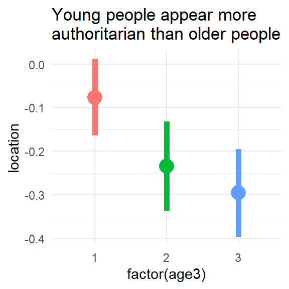

In the plot, the estimates represent means and 95% confidence intervals. The X axis represents the respondent’s age tercile, with larger values indicating older respondents. The Y axis represents the respondent’s location on the latent trait, which scholars typically label, “authoritarianism.”

Or we can use an OLS regression to see if authoritarianism varies with age:

Show code

ols <- lm(location ~ factor(age3), data = anes_locations_4) 
summary(ols)

Call:
lm(formula = location ~ factor(age3), data = anes_locations_4)

Residuals:
     Min       1Q   Median       3Q      Max 
-3.15427 -1.07630 -0.06981  0.95589  2.53532 

Coefficients:
              Estimate Std. Error t value Pr(>|t|)   
(Intercept)   -0.07617    0.04889  -1.558  0.11932   
factor(age3)2 -0.15775    0.06961  -2.266  0.02351 * 
factor(age3)3 -0.21924    0.06969  -3.146  0.00167 **
---
Signif. codes:  0 '***' 0.001 '**' 0.01 '*' 0.05 '.' 0.1 ' ' 1

Residual standard error: 1.691 on 3516 degrees of freedom
  (631 observations deleted due to missingness)
Multiple R-squared:  0.002998,  Adjusted R-squared:  0.002431 
F-statistic: 5.287 on 2 and 3516 DF,  p-value: 0.005096

Consistent with the figure, the model suggests that people in age groups 2 and 3 are less authoritarian than the youngest age group. We can also compare the authoritarianism levels of groups 2 and 3 with the car::linearHypothesis() function:

Show code

car::linearHypothesis(ols, "factor(age3)2 = factor(age3)3")

Linear hypothesis test

Hypothesis:
factor(age3)2 - factor(age3)3 = 0

Model 1: restricted model
Model 2: location ~ factor(age3)

  Res.Df   RSS Df Sum of Sq      F Pr(>F)
1   3517 10053                           
2   3516 10051  1    2.1959 0.7682 0.3808

The small F statistic indicates that groups 2 and 3 do not differ significantly in their authoritarianism.

We can compare these estimates to those we would have obtained had we relied on the off-the-shelf scale without first establishing measurement equivalence:

Show code

anes_naive <- anes_sub  %>% 
  mutate(n_items = 
           4L - 
           (is.na(auth_respect) + 
           is.na(auth_manners) + 
           is.na(auth_obed) + 
           is.na(auth_behave)))  %>%
  mutate(sum_items = 
           select(., auth_respect, auth_manners, auth_obed, auth_behave)  %>% 
           rowSums(na.rm = TRUE)
         )  %>% 
  mutate(off_the_shelf = scale(sum_items/n_items))

# fit "naive" regression 
ols_naive <- lm(off_the_shelf ~ factor(age3), data = anes_naive) 
summary(ols_naive)

Call:
lm(formula = off_the_shelf ~ factor(age3), data = anes_naive)

Residuals:
     Min       1Q   Median       3Q      Max 
-1.72232 -0.81210 -0.05625  0.69961  1.45546 

Coefficients:
              Estimate Std. Error t value Pr(>|t|)    
(Intercept)   -0.09153    0.02886  -3.172 0.001529 ** 
factor(age3)2  0.15436    0.04109   3.756 0.000175 ***
factor(age3)3  0.12288    0.04114   2.987 0.002836 ** 
---
Signif. codes:  0 '***' 0.001 '**' 0.01 '*' 0.05 '.' 0.1 ' ' 1

Residual standard error: 0.998 on 3516 degrees of freedom
  (631 observations deleted due to missingness)
Multiple R-squared:  0.004478,  Adjusted R-squared:  0.003912 
F-statistic: 7.908 on 2 and 3516 DF,  p-value: 0.0003744

For comparison, here is a summary of the corrected estimates and the off-the-shelf estimates:

Show code

htmlreg(
  list(ols_naive, ols),
  custom.model.names = c("Off-the-shelf", "Corrected"),
  bold = 0.05,
  stars = 0.05,
  caption = "The corrected scale suggests older people have lower values of the latent trait. The off-the-shelf scale suggests the opposite."
  
    )

The corrected scale suggests older people have lower values of the latent trait. The off-the-shelf scale suggests the opposite.

	Off-the-shelf	Corrected
(Intercept)	-0.09*	-0.08
	(0.03)	(0.05)
factor(age3)2	0.15*	-0.16*
	(0.04)	(0.07)
factor(age3)3	0.12*	-0.22*
	(0.04)	(0.07)
R2	0.00	0.00
Adj. R2	0.00	0.00
Num. obs.	3519	3519
*p < 0.05

The table above shows that researchers using the off-the-shelf scale would come to opposite conclusions than would researchers using the corrected scale on which the three groups are now comparable. This difference occurs because the nuisance dimension has been removed, not because the scale has changed fundamentally in meaning. Though the results change considerably after correction, the corrected scale is nonetheless strongly correlated with the off-the-shelf scale:

Show code

the_cor <- anes_locations_4  %>% 
  select(case_id, corrected = location)  %>% 
  left_join(anes_naive)  %>% 
  select(off_the_shelf, corrected)  %>% 
  cor(use = "pairwise.complete.obs")

the_cor

              off_the_shelf corrected
off_the_shelf     1.0000000 0.9759355
corrected         0.9759355 1.0000000

The two scales are correlated at \(\hat{\rho} =\) 0.98. Therefore, the corrected scale retains almost all of the content of the off-the-shelf scale, except the bias associated with DIF by age.

6. Key Points

This analysis demonstrates several key points:

• The data used to construct the 2016 ANES Authoritarianism scale exhibit DIF by age.
• Without correction, the scale will lead to biased conclusions about the relationship between the Authortarianism latent trait and age.
• This problem can be addressed using the sequential Rasch method outlined here.
• The corrected scale retains most of the information of the uncorrected, off-the-shelf scale (\(\hat{\rho} =\) 0.98), but purges bias associated with DIF by age.

Keep in mind,

• DIF is often interesting substantively. Though it must be removed to avoid biased conclusions, it should also be examined to see if it illuminates meaningful qualitative differences between groups.
• By examining DIF within these data, this tutorial focuses on identifying removing the influence of unintended “nuisance” dimensions that bias group comparisons by impinging on the measurement occasion. It does not focus on establishing the content validity of a scale, which is also essential for meaningful group comparisons.

More Information

For more information, find links to the full article (Pietryka & Macintosh, 2022), supporting info, and replication materials below.

Downloads	External Links
article (pdf)	replication materials
supporting info (pdf)	DOI:10.1086/715251
BibTeX citation

Session Information

See below for information about the operating system, software, and packages used for this post.

Show code

sessionInfo()

R version 4.2.3 (2023-03-15 ucrt)
Platform: x86_64-w64-mingw32/x64 (64-bit)
Running under: Windows 10 x64 (build 19045)

Matrix products: default

locale:
[1] LC_COLLATE=English_United States.utf8 
[2] LC_CTYPE=English_United States.utf8   
[3] LC_MONETARY=English_United States.utf8
[4] LC_NUMERIC=C                          
[5] LC_TIME=English_United States.utf8    

attached base packages:
[1] stats     graphics  grDevices utils     datasets  methods  
[7] base     

other attached packages:
 [1] texreg_1.38.6     kableExtra_1.3.4  broom_1.0.4      
 [4] ggplot2_3.4.3     TAM_4.1-4         CDM_8.2-6        
 [7] mvtnorm_1.1-3     readr_2.1.4       purrr_1.0.2      
[10] tibble_3.2.1      tidyr_1.3.0       dplyr_1.1.2      
[13] htmltools_0.5.5   icons_0.2.0       fontawesome_0.5.0
[16] glue_1.6.2       

loaded via a namespace (and not attached):
 [1] Rcpp_1.0.10       svglite_2.1.1     rprojroot_2.0.3  
 [4] digest_0.6.31     utf8_1.2.3        mime_0.12        
 [7] R6_2.5.1          backports_1.4.1   evaluate_0.20    
[10] highr_0.10        httr_1.4.7        pillar_1.9.0     
[13] rlang_1.1.1       rstudioapi_0.14   car_3.1-2        
[16] jquerylib_0.1.4   rmarkdown_2.21    labeling_0.4.2   
[19] webshot_0.5.4     stringr_1.5.0     munsell_0.5.0    
[22] compiler_4.2.3    xfun_0.38         pkgconfig_2.0.3  
[25] systemfonts_1.0.4 downlit_0.4.2     tidyselect_1.2.0 
[28] bookdown_0.33     polycor_0.8-1     fansi_1.0.4      
[31] viridisLite_0.4.1 crayon_1.5.2      tzdb_0.3.0       
[34] withr_2.5.0       MASS_7.3-58.2     rappdirs_0.3.3   
[37] grid_4.2.3        jsonlite_1.8.7    gtable_0.3.3     
[40] lifecycle_1.0.3   magrittr_2.0.3    scales_1.2.1     
[43] carData_3.0-5     cli_3.6.1         stringi_1.7.12   
[46] cachem_1.0.7      farver_2.1.1      xml2_1.3.5       
[49] bslib_0.4.2       admisc_0.31       generics_0.1.3   
[52] vctrs_0.6.3       distill_1.5       forcats_1.0.0    
[55] tools_4.2.3       hms_1.1.3         abind_1.4-5      
[58] parallel_4.2.3    fastmap_1.1.1     yaml_2.3.7       
[61] colorspace_2.1-0  rvest_1.0.3       memoise_2.0.1    
[64] haven_2.5.2       knitr_1.42        sass_0.4.5       
[67] postcards_0.2.3  

---

1. see: (1) Andrich, David and Curt Hagquist. 2012. “Real and Artificial Differential Item Functioning.” Journal of Educational and Behavioral Statistics, 37(3): 387–416. (2) Andrich, David and Curt Hagquist. 2015. “Real and Artificial Differential Item Functioning in Polytomous Items.” Educational and Psychological Measurement, 75(2): 185–207.↩︎

2. If one wishes to take a more conservative approach against DIF, one could instead separate all groups that exhibit non-negligible differences.↩︎

3. Engelhardt, Andrew M., Stanley Feldman, and Marc J. Hetherington. “Advancing the Measurement of Authoritarianism.” Political Behavior. https://doi.org/10.1007/s11109-021-09718-6.↩︎